(See this Wikipedia article for a quick review of Power law fits.)
So linear curve fits are easy in MATLAB — just use p=polyfit(x,y,1), and p(1) will be the slope and p(2) will be the intercept. Power law fits are nearly as easy. Recall that any data conforming to a linear fit will fall along a given by the equation [latex]y=kx+a[/latex]
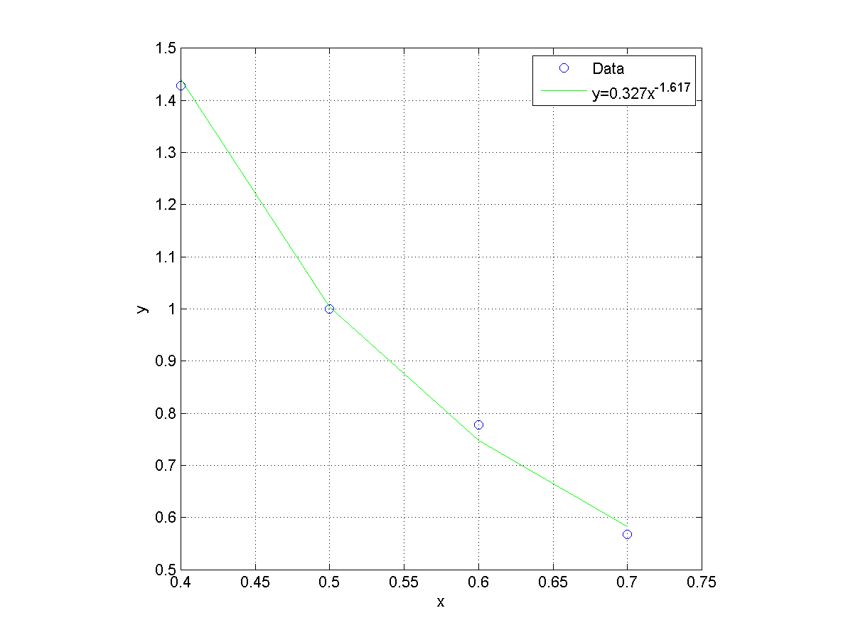
Similarly, any data conforming to a power law fit will fall along a curve given by the equation [latex]y=ax^k[/latex]
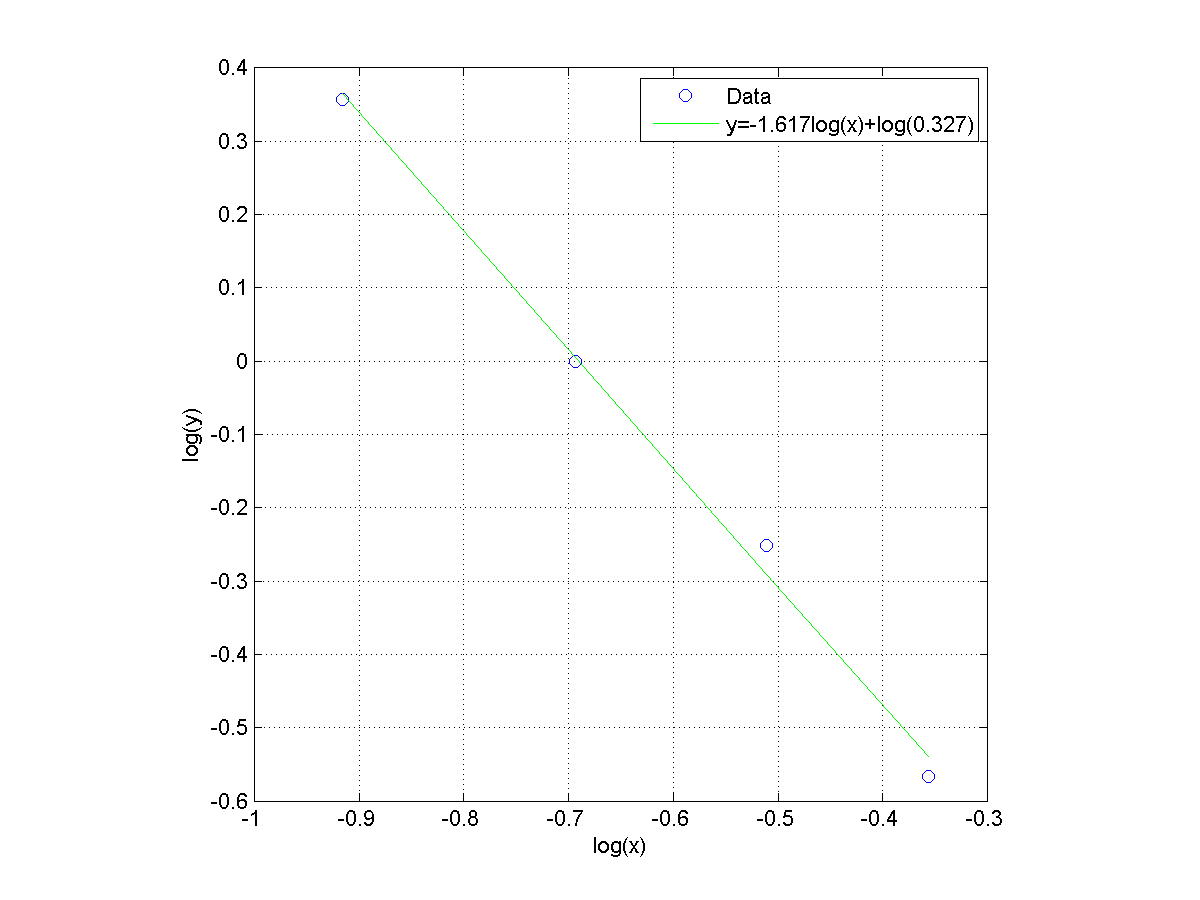
If we plot the second equation on log-log axes, it describes a family of straight lines. Put another way, if we take the log of y and x and plot them on linear axes, those logs will fall along a straight line. So all we need to do in MATLAB is to take the log of both x and y, and then let polyfit do its job. For example:
clear all
close all
x=[0.4 0.5 0.6 0.7];
y=[1.429 1 0.778 0.5675];
logx=log(x);
logy=log(y);
p=polyfit(logx,logy,1);
plot(logx,logy,'bo');
axis equal square
grid
xlabel('log(x)');
ylabel('log(y)');
k=p(1);
loga=p(2);
a=exp(loga);
hold on; plot(logx,k*logx+loga,'g')
legend('Data',sprintf('y=%.3f{}log(x)+log(%.3f)',k,a));
figure
plot(x,y,'bo');
xlabel('x');
ylabel('y');
axis equal square
grid
hold on; plot(x,a*x.^k,'g')
legend('Data',sprintf('y=%.3f{}x^{%.3f}',a,k));
returns the following figures:
This little piece of code help me a lot, thank you!!
That was really useful.
Thank you
That was extremely helpful. One question: what does %.3f mean?
Fixed-point format, with 3 digits after the decimal symbol. See Mathworks’ sprintf documentation for more information.
I want the curve fitting equation like ..
y=a ±(error in a ) * x^b±(error in b)