One of the faculty has some axisymmetric diffusion simulation code written in Excel and VBA. He didn’t think his 2D graphs of chemical concentration along a particle’s radius would be suitable for an audience he’d be presenting to, and that they’d be better served seeing an animation of how the concentration varied over time and position. Here’s where we started, more or less:
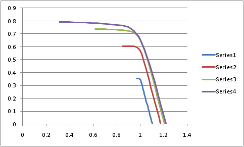 and I had to be informed that the horizontal axis was radius from the particle center (normalized to 1 for the original particle radius), the vertical axis was something resembling a chemical concentration or composition, and that each line represented a different point in time. Excel’s default line thickness and other design choices bother me, so let’s go ahead and redo that graph in Matlab:
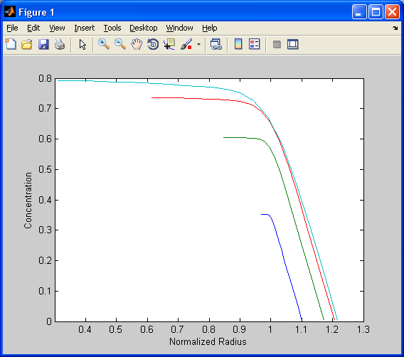 As it turns out, the concentration isn’t undefined closer to the particle center. Since this is a differential equation solution, we assume that the concentration is identically 1 everywhere from the center to the inside boundary radius. So, the total graphs of concentration versus distance should be:
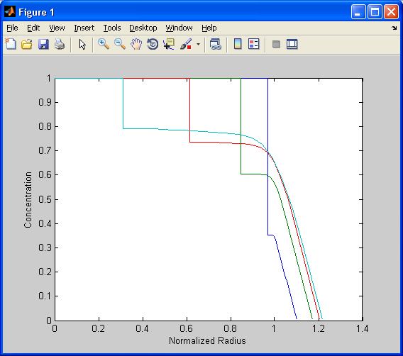 which makes it a bit more explicit that we have a lump of pure material that gets gradually eaten away by its surroundings and becomes smaller.
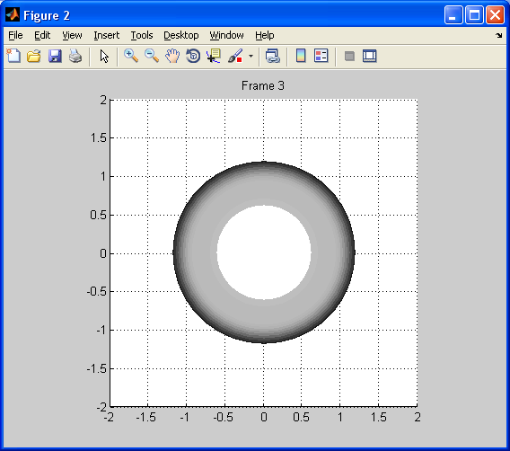
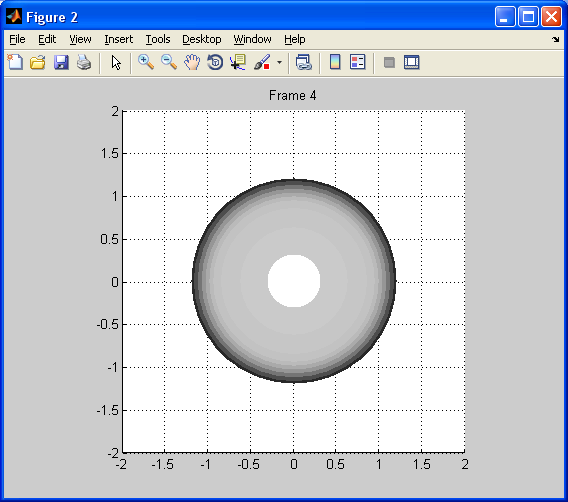
Now to convert that line graph into an axisymmetric representation. Mathworks already outlined how to do a basic mesh plot in polar coordinates, so all we have to do is adapt their instructions to our data. We don’t actually have to work out all the complex math, we just need to make a matrix for each point in time of equal size to the X and Y matrices created by meshgrid and pol2cart. Each column of this matrix should be the original Y data from Excel for that particular time, and the repmat function takes care of that. The resulting mesh plot of the last time step examined then looks like: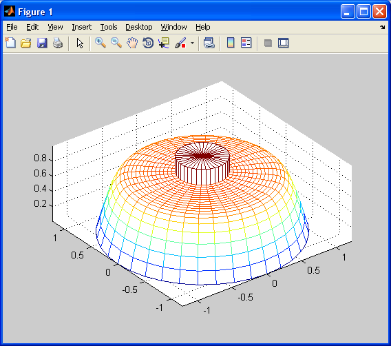 All that’s left now is to:
- Change the mesh plot to a surface
- Remove the edge colors on each patch (so we have just the patch colors, not the edges)
- Reorient our view to top-dead-center (like how we see the original material under the electron microscope)
- Change the colormap to grayscale (like how we see the original material under the electron microscope)
- Convert each plot into a frame of a video file with avifile and addframe.
Here’s the code:
clear all
close all
data=[ ...
    0.968682635	0.352941008	0.847944832	0.604846848	0.614770029	0.736745905	0.309963787	0.792192895
    0.975319116	0.352912882	0.864179809	0.60473259	0.644348798	0.736479267	0.355305164	0.791705755
    0.981955598	0.352843355	0.880414786	0.604508532	0.673927568	0.735967459	0.400646542	0.790820863
    0.988592079	0.352367206	0.896649763	0.604178754	0.703506337	0.735228449	0.445987919	0.789595717
    0.99522856	0.349314226	0.91288474	0.603743855	0.733085106	0.734277487	0.491329297	0.788068624
    1.001865042	0.339595849	0.929119717	0.603165414	0.762663875	0.733127586	0.536670674	0.786265735
    1.008501523	0.322069418	0.945354694	0.60215826	0.792242645	0.731789334	0.582012051	0.78420522
    1.015138005	0.300279218	0.961589671	0.599529003	0.821821414	0.730264749	0.627353429	0.781899808
    1.021774486	0.277475921	0.977824648	0.592185016	0.851400183	0.728502808	0.672694806	0.779357749
    1.028410967	0.254600132	0.994059625	0.575269388	0.880978952	0.726191443	0.718036184	0.776577069
    1.035047449	0.23173444	1.010294602	0.544925458	0.910557722	0.722114592	0.763377561	0.773500341
    1.04168393	0.208878058	1.026529579	0.501653986	0.940136491	0.712945073	0.808718939	0.76979412
    1.048320411	0.186029734	1.042764556	0.449999723	0.96971526	0.692373171	0.854060316	0.76410296
    1.054956893	0.163188804	1.058999533	0.394837376	0.999294029	0.652709252	0.899401693	0.752396638
    1.061593374	0.140354946	1.075234511	0.338837483	1.028872799	0.589603167	0.944743071	0.72609778
    1.068229856	0.117527765	1.091469488	0.282806787	1.058451568	0.505896949	0.990084448	0.672977986
    1.074866337	0.094706669	1.107704465	0.226853501	1.088030337	0.4097422	1.035425826	0.583653876
    1.081502818	0.071890988	1.123939442	0.170955144	1.117609106	0.308800318	1.080767203	0.459732008
    1.0881393	0.049079865	1.140174419	0.115095194	1.147187876	0.206932201	1.12610858	0.313724213
    1.094775781	0.026271856	1.156409396	0.059265944	1.176766645	0.10513866	1.171449958	0.159292943
    1.101412262	0.003483628	1.172644373	0.00345515	1.206345414	0.003440781	1.216791335	0.003438214
];
nFrames=size(data,2)/2; % due to 2 columns of data per frame
revgray=colormap(gray);
% 64x3 array of gray RGB values ([1 1 1] -> white and high values,
% [0 0 0] -> black and low values) -- gray is a built-in colormap
% revgray=revgray(size(revgray,1):-1:1,:);
% Reverse order of rows in revgray: results in a 64x3 array of gray RGB
% values ([0 0 0] -> black and high values, [1 1 1] -> white and low
% values)
fig=figure;
aviobj=avifile('diffusion.avi','FPS',15,'Quality',100);
for n=1:nFrames
    radius=data(:,n*2-1);
    concentration=data(:,n*2);
    % Add an extra data point at r=0 and r=min(r)
    radius=[0; min(radius); radius];
    concentration=[1; 1; concentration];
    % Build a polar grid (from Matlab help, "Displaying Contours in Polar
    % Coordinates")
    [th,r] = meshgrid((0:10:360)*pi/180,radius);
    [X,Y] = pol2cart(th,r);
    Z = X+i*Y; % For the purposes of polar math, abs(Z) is basically r.

    f=repmat(concentration,1,size(Z,2));
    % repmat(X,nr,nc) repeats X by nr rows and nc columns. size(Z,2)
    % returns the number of columns in Z. We end up with an array of
    % identical size to Z. f ends up being 1*concentration for all theta,
    % and concentration only varies with respect to r.

    surf(X,Y,abs(f),'EdgeColor','none');
    axis([-2 2 -2 2 0 1]);
    colormap(revgray);
    view(2);
    axis equal;
    title(sprintf('Frame %d',n));
    F=getframe(fig);
    aviobj=addframe(aviobj,F);
    pause(0.1);
end
aviobj=close(aviobj);
and the resulting still images and video: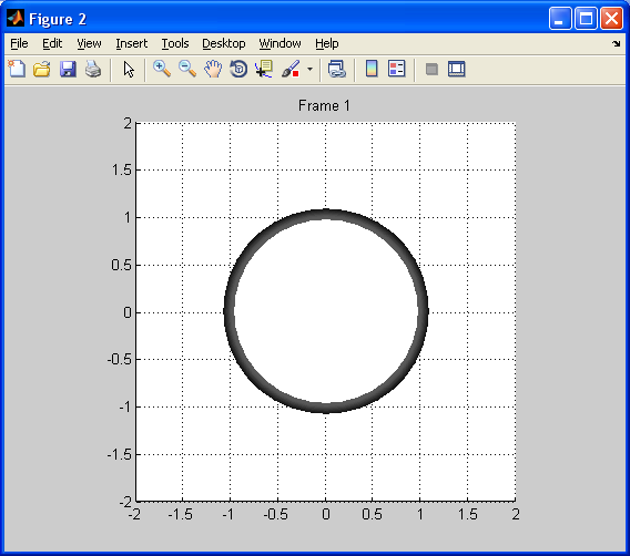

Diffusion video (very short, 4 frames at 1 fps, may or may not play directly in the browser, so just download it)
Mike,
Where do you see this being used in a practical application.
Hello ,
I’m looking for a low pass filter program with ms office or so basic software .Have you got any idea about this???
Regards.
(Sorry for the delay, just went through the pending comments folder.)
Unless Office is a requirement for some reason, you’ll be better off doing filters in Octave (free) or MATLAB (not). Doing them in Excel would basically require you to write VBA code to convert a series of cells into the filtered result. You’d need all the equations for filtering, and it’d be a lot of effort for little result in most cases.