Running Chemistry Simulations on the TNTECH HPC Cluster

The two most commonly used HPC applications in chemistry research on our campus are Gaussian ’09 (for ab initio and semi-empirical quantum mechanics), and NAMD (for classical molecular dynamics). To manage the queue of different computational jobs on the cluster, it makes use of the SLURM Workload Manager. In addition to the files containing your structure, parameters and/or topology, you will need an input script which essentially tells the HPC how much CPU time you are requesting, how many nodes and CPUs you want to use, as well as where the NAMD or Gaussian executables are.

Please contact dcashman@tntech.edu or the HPC cluster administrator, renfro@tntech.edu, if you have any questions or issues in running jobs on the HPC cluster.

Running a Gaussian ’09 Simulation

To initiate a job using Gaussian ’09, you will need Gaussian ’09 input file. This file usually ends with the suffix *.com and contains the method, basis set and internal coordinates of your system. If you used GaussView to generate this file, it will end with *.gjf, but the format is identical. More information on Gaussian input files is here (note that input for Gaussian ’09 and Gaussian ’16 use essentially the same commands).

You should upload all of the following files to the Tennessee Tech HPC cluster using the IP address provided to you by the HPC administrator (for security reasons, the IP address is not included here). Next, create a subdirectory in your home directory on the cluster for your simulation files to be contained in. Upload all simulation files to that directory using SCP. In that subdirectory, create a new file called g09_simulation.sh. This file should contain the following lines:

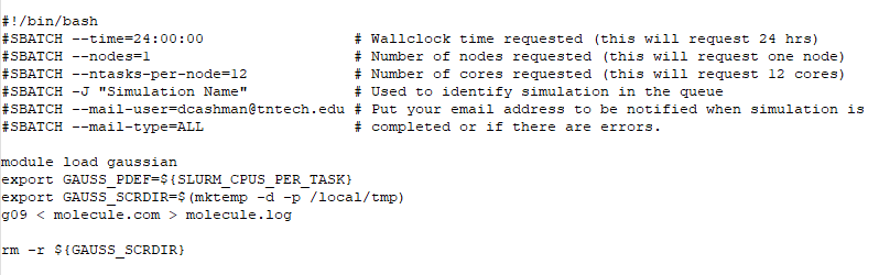
Save your simulation input file and ensure that the file is executable by typing chmod 755 g09_simulation.sh (or whatever your script is named). Please note that the cluster has 40 nodes with 28 CPU cores on each node. Gaussian ’09 does not scale well to multiple nodes or more than 12 or 16 CPUs. If you request more CPU cores than that, you may find that the software is not utilizing all cores (so you should not request more than 12 or 16 CPU cores).

To begin running your simulation, type sbatch g09_simulation.sh at the prompt. You may confirm the status of your job by typing squeue -u username. You may also view the HPC cluster queue from any workstation on campus at bright80.hpc.tntech.edu/slurm.

Note that some Gaussian ’09 calculations require more temporary scratch space on the hard disk (such as MP2 calculations). If you are having issues with jobs terminating because of lack of scratch space, you may wish to change the GAUSS_SCRDIR above a temporary directory in your home directory. To do so, type mkdir tmp in your home directory, and change the GAUSS_SCRDIR to ~username/tmp.

Running a NAMD Simulation

To initiate a simulation using NAMD, you will need the following structure/parameter files:

  • PDB coordinate file of system of interest (if generated using MOE 2022, this file may end with *.coor)
  • Protein Structure File (PSF) containing force field information
  • Parameter file (PAR) containing all of the numerical information for evaluating forces and energies.
  • NAMD Configuration File (conf) containing the parameters of the molecular dynamics simulation itself. If you’re using MOE 2022, this will be generated from the software itself. Please see the NAMD Tutorial for more information about what this file should contain.

You should upload all of the following files to the Tennessee Tech HPC cluster using the IP address provided to you by the HPC administrator (for security reasons, the IP address is not included here). Next, create a subdirectory in your home directory on the cluster for your simulation files to be contained in. Upload all simulation files to that directory using SCP. In that subdirectory, create a new file called namd_simulation.sh. This file should contain the following lines:

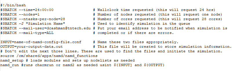
Save your simulation input file and ensure that the file is executable by typing chmod 755 namd_simulation.sh (or whatever your script is named). Please note that the cluster has 40 nodes with 28 CPU cores on each node. If you wish to run a simulation on multiple nodes, set (for example) nodes=2 to run on 56 CPU cores total (don’t change the ntasks-per-node variable).

To begin running your simulation, type sbatch namd_simulation.sh at the prompt. You may confirm the status of your job by typing squeue -u username. You may also view the HPC cluster queue from any workstation on campus at bright80.hpc.tntech.edu/slurm.

There is a second cluster containing a small number of AMD Ryzen CPUs. As this is not 100% in production yet, you should contact dcashman@tntech.edu if you are interesting in utilizing these resources.

Special Note on HPC Cluster Resources

Please note that this is a shared resources by many users throughout Tennessee Technological University. As such, you should be cognizant of that fact and not “hog” the system. While the maximum number of nodes you can request is 40, doing so will likely mean your job will be waiting in the queue a long time because you’re requesting 100% of the HPC cluster. If you do that, you will likely be contacted by the HPC Cluster administrator.

You should look at the current queue on the cluster before submitting any job and adjust your request for resources accordingly. As a general rule of thumb, Gaussian ’09 jobs should never be requesting more than 1 node or 16 CPU cores, and NAMD jobs should be limited to three to five nodes (84 to 140 CPU cores). You also may request more than 24 hours (several days of time is allowed). Be aware that the more resources that you request may result in a longer queueing time before your job runs because it may take longer for resources to be freed up by other jobs.

Posted in Tutorials | Comments Off on Running Chemistry Simulations on the TNTECH HPC Cluster

Tutorial: Windows vs. UNIX/Linux File Formatting Tips

For the most part, files generated in Windows will be compatible and readable on a UNIX/Linux system. One of the first key things for users to understand is that UNIX filenames are case-sensitive, while Windows filenames are not. So there is a difference between filename.txt and Filename.txt in UNIX. For this reason, I recommend leaving the CAPS LOCK key off for most activities on UNIX systems.

It is also important to remember that UNIX filesystems and many programming languages used in scientific computing will recognize a a filename containing a space, ” “, as delimiting between two filenames. If you do have a space in a filename, you will have to “escape” the space using the escape character preceding the space. The escape character is a backslash (\). For example, to edit a file named, “file name.txt“, you will have to type, “gedit file\ name.txt“. For this reason, it would be easier to try to remember to not include spaces in filenames. Use the underscore (_) character instead. This way, “file name.txt” would become, “file_name.txt“.

Most Windows files will work fine in most programs running on UNIX and Linux. However, if you are running a file through some software programs, you may encounter issues with differences in how Windows treats an end of line with some extra characters. These extra characters may cause errors in some programs. If you encounter this issue, you can run a simple awk command at the UNIX shell to handle this error:

awk ‘{ sub(“\r$”, “”); print }’ <filename>.sh > <filename>_n.sh

This will remove the end of line characters from the Windows file and create a new UNIX formatted file with a _n after the filename (the original file will be preserved.

Posted in Tutorials | Leave a comment

Tutorial: Printing on the Poster Printer in LSC-2335

HP DesignJet T530 Poster Printer in LSC-2335

The HP DesignJet T530 is a high quality, large format printer capable of printing up to 36″ wide for scientific posters. This printer is available to faculty and student researchers in the Department of Chemistry. The printer is located at the opposite end of the computer modeling laboratory near the windows. There is a computer running Microsoft Windows on the right side near the back of the room to use for printing posters.

Poster Printing Instructions

  • The first step in printing your poster is to save your poster in Microsoft Powerpoint format. Be sure to edit the Page Layout and set the dimensions of the page to 48″ x 36″ — landscape. Once your poster is complete, it is recommended to print first to a standard printer in landscape mode to ensure that the fonts appear normal and there are no glitches. This serves as a proof. You can also print to PDF format for proofreading. Please DO NOT send un-proofread documents to the HP DesignJet T530 printer to avoid wasting paper and ink.
  • Login to the Microsoft Windows computer in the back of the room using your TNTECH network credentials and copy your poster to the Desktop. You can copy your powerpoint file by: (a) emailing the file to yourself and logging into your email account; (b) copying the file from a thumbdrive inserted into the computer’s USB port; or (c) opening the command prompt and using SCP to copy the file from another networked computer.
  • Be sure to turn the HP DesignJet T530 printer ON by pressing the power button on the left side near the console screen. You should also reach under the printer and pull out the bar underneath to open the poster bin so that your poster will be collected in the bin and does not fall on the ground after it is printed.
  • Open Microsoft Powerpoint and load your poster. Click on FILE > PRINT. Select the HP DesignJet T530 as the printer in this menu. Click on Printer Properties to select the paper size. Assuming your poster is 48″ x 36″ in size as described above, select Arch E under Document Size and Roll under Paper Source. Click OK to go back to the main print menu.
  • Back in the main print menu, if you are ready to print and have proofread your poster, click the PRINT button at the top and the poster will be sent to the printer.
  • Once your poster is printed, log out of the computer, turn the HP DesignJet T530 OFF, and push the bar towards the back of the printer underneath to stow the output bin.

Poster Design? If you are new to designing and editing posters, you may wish to download the poster template provided below for easy editing. The powerpoint file is set to a page size of 48″ x 36″.

Note: If the printer is out of ink, please DO NOT replace the ink cartridges yourself. Please contact Dr. Derek Cashman so that new ink cartridges can be installed and replacements can be ordered.

Questions? Contact Dr. Derek Cashman or Dr. Amanda Carroll.

Posted in Tutorials | Leave a comment

Molecular Modeling Laboratory Now Open in LSC

The molecular modeling laboratory is now open in the new Laboratory Science Commons, room 2335. This laboratory is a shared research resource with eight Linux workstations and a variety of molecular modeling software such as MOE 2020, NAMD, VMD, Gaussian ’09, Gromacs, and more. The facility also features a poster printer and technology that is available for classroom teaching and demonstrations of molecular modeling and computational chemistry. Additional Linux workstations are currently on order, as well as future color printing and 3D printing capabilities.

Access to the room is via card access. If you would like to use these systems for research and be added to the access control for this facility, or you have any questions on any of the resources available, please contact Dr. Derek Cashman.

Posted in Announcements, Uncategorized | Leave a comment

Chemistry Demonstration: Shaving Cream Swirls

Introduction

The experiment demonstrates the interactions between hydrophobic and hydrophilic substances. Hydrophobic substances repel water – the name comes from the Greek word, “Hydros”, for water, and, “phobos”, for fear. Hydrophilic substances (the Greek stem, “philic”, means “love”) attract, or love, water.

A polar molecule has a separation of positive and negative charges, while a non-polar molecule has no areas of prevalent positive or negative charges (it is neutral). Water is a polar molecule, having positive charge around the hydrogen and a negative charge around the oxygen. Because water is polar, other polar molecules will be attracted to it; these are the molecules we describe as hydrophilic. Conversely, hydrophobic molecules are non-polar/non-charged.

Soap molecules are very interesting in that they contain both hydrophobic portions and hydrophilic portions. We refer to these molecules as AMPHIPATHIC. These molecules typically have a polar head and a long, hydrophobic tail. Shaving cream is a foam consisting of molecules of soap and air.

Food coloring consists of dye molecules that are dissolved in water, so they must be hydrophilic. When these dyes are added to shaving cream, the dye molecules can only interact with the polar heads of the soap molecules, and not with the hydrophobic tails. This therefore limits their mobility. Molecules in paper are composed of molecule of cellulose (a polymer of glucose). Cellulose contains multiple polar hydroxyl functional groups that can interact readily with water, so paper is very hydrophilic. Because both the food coloring dyes and paper molecules are hydrophilic, they will interact readily with one another and the dyes will spread easily across the paper to form very colorful patterns in a much different way than they interacted with the shaving cream. This creates a marbling effect on the paper that is clearly distinct from the pattern seen on the shaving cream.

Materials

  • Shaving Cream
  • Food Coloring
  • Squeegees
  • Wax Paper
  • Small pieces of card stock paper (3×5 index cards)
  • Toothpicks
  • Paper plates (optional)

Procedure

  1. Place a large sheet of wax paper on a solid surface (table) to make it easier to clean up.
  2. Place a small mound of shaving cream on the wax paper or a paper plate. Add three to four drops of food coloring to the shaving cream and swirl it with a toothpick. Be careful not to overswirl. If all of the colors blend together into a new color the final product will not be as attractive.
  3. Place a 3×5 index card on the shaving cream mound and press down lightly. Remove the card and use a squeegee to remove excess shaving cream. Observe the marbled paper product!
  4. The mound of shaving cream can be re-used by re-swirling it. You can add a new drop of food coloring or leave it as-is. You can color the back of their card or another card. Swirl the colors around some more to see how it chages the marbled pattern.

Safety

This experiment is relatively safe. All products can be purchased from a grocery store and there are no major safety issues.

Disposal of Waste Products

No special requirements. Everything can be discarded through normal disposal procedures. Mix the shaving cream with water and flush down the drain.

TTU Chemistry students demonstrating shaving cream swirls at the Fall Fun Fest, 2015, in Cookeville.
TTU student demonstrating the final product of the shaving cream swirl experiment.
Posted in Demos, Uncategorized | Leave a comment

Chemistry Demonstration: PVA Slime

Introduction

Multi-colored slime can be created using a solution of poly-vinyl alcohol (PVA) and borax. This experiment demonstrates the ability of borax to form chemical cross-links between molecules of the PVA polymer. The chemical structures below show a molecule of the PVA polymer on the left and a molecule of borax (borate ion) on the right.

When these molecules are mixed together, hydrogen bonds are formed between the hydroxyl groups of both the PVA and borate ion. This “sticks” them together and creates the slimy texture to the mixture.

Slime is a non-Newtonian fluid that dilate, or expand, under stress. Similar substances with these properties include quicksand, starch solutions and Silly Putty. Dilatant materials tend to have some unusual properties.

If you slowly pull on the material, it will flow and stretch. If you are very careful, you can form a thin film. But if you pull sharply (inducing high stress), the material will break. If you pour the material from its container and tip the container slightly upwards, the gel will siphon itself.

Materials

  • 2 L soda bottles (remove the label)
  • Small disposable cups
  • Plastic spoons or wooded stirrers
  • 4% Poly-Vinyl Alcohol (PVA) solution
  • 4% Borax solution
  • Food coloring
  • ZipLoc Bags
  • Wax Paper or Tarp for easy cleanup
  • 0.5 M Hydrochloric Acid (HCl) (optional)
  • 0.5 M Sodium Hydroxide (NaOH) (optional)

Procedure

  1. Prior to the demonstration, prepare the Poly-Vinyl Alcohol (PVA) solution by adding 4 g of PVA to 100 mL of hot, deionized water (70°C). You may use a microwave to heat the water. Put the 4% PVA solution into 2 L soda bottles for storage. Prepare the 4% borax solution by mixing 4 g Na2B4O7 in 100 mL of deionized water.
  2. At the demonstration, perform all mixing of PVA and borax on the wax paper or tarp. You will mix the two solutions together in a 10:1 (PVA:borax) ratio in the small cups provide. Add two to four drops of food coloring of the desired color. Mix well using the plastic spoon or wooden stirrers. A gel should form immediately.
  3. Demonstrate the flexibility and pliability of the gel.
  4. Optional: Adding acid (HCl) to the slime breaks the crosslinking and produces a liquid with lower viscosity. If you add a base (NaOH), the process is reversed and the slime is regenerated.
  5. The slime can be taken home by storing it in a ZipLoc bag.

Safety

Wear eye protection and latex gloves when handling slime.

Disposal of Waste Products

All waste products may be safely disposed of in the garbage.

Making PVA Slime at the 2013 Fall Fun Fest in Cookeville.
Posted in Demos, Uncategorized | Leave a comment

Chemistry Demonstration: Molecular Modeling with Candy

Introduction

This is a fun demonstration that teaches students how to build simple molecular models using colored candies. It is relatively simple to prepare and set up, and easy to maintain. The basic principles of building small molecular models of organic compounds can be easily demonstrated. The basics of single, double and triple bonds can be demonstrated.

Materials

  • Toothpicks
  • Soft, jellied candies of a variety of colors
  • A large bowl or ziploc bags to contain the candy atoms
  • 3×5 Index Cards
  • Markers or Sharpies

Procedure

  1. Place all of the jellied candies in a large bowl or ZipLoc bags. You may opt to separate the candies by color, but it is not necessary.
  2. Place the toothpicks on the table for easy access.
  3. Decide ahead of time a small collection of potential models for participants to construct, and draw their names and chemical structures on the 3×5 index cards. The best molecules to build in this project are small organic molecules (the simpler the better). Planar aromatic compounds also work the best, since they can be built and rested on the table for stability (the candies are often heavy enough to not stay upright in, for example, a tetrahedral carbon atom).Examples of good molecules to use for this demonstration include:
    • Water (H2O)
    • Acetylene (C2H2)
    • Carbon Dioxide (CO2)
    • Carbonic Acid (H2CO3)
    • Ethane
    • Ethanol (CH3CH2OH)
    • Ethylene
    • Glucose or Fructose (C6H12O6)
    • Methane
    • Propane
    • Ribose
    • 20 Amino Acids
    • Palmitic Acid
    • alpha-Linoleic Acid
    • Cyclohexane (boat and chair conformations?)
  4. A single toothpick represents a single bond, two toothpicks represents a double bond, and three toothpicks represent a triple bond.

Safety

This experiment is relatively safe. It uses edible candies. However, because the candies will tend to be handled by many people, eating them is not recommended and should be discouraged. Also, the toothpicks can be sharp, so care should be taken to avoid poking oneself with them.

Disposal of Waste Products

No special requirements. Everything can be discarded through normal disposal procedures.

A candy molecule of a small, aromatic compound.
Posted in Demos, Uncategorized | Leave a comment

Chemistry Demonstration: Molecular Modeling with Avogadro

Introduction

This is a simple and fun, hands-on activity that demonstrates the basic concepts of computer-based molecular modeling. Using molecular mechanics, small molecules may be modeled by treating the atoms as balls and the bonds connected them as springs. We can then use a set of equations, which we refer to as a force field to place these atoms in the correct geometrical arrangement and calculate a relative energy that we can use to compare different conformations of these molecules.

The basic components of a typical molecular mechanics force field include:

Erelative = Ecovalent interactions + Enon-covalent interactions

The covalent and non-covalent interactions can further be broken down into the following components:

Ecovalent interactions = Ebond-stretching + Eangle-bending + Etorsion

Enon-covalent interactions = Eelectrostatic + Evan der Waal’s

The equations used for the covalent interactions are Hook’s law (spring harmonics). Equations used for the electrostatic interactions is Coulomb’s law, and the equations used for the van der Waal’s component is the 6-12 Lennard-Jones potential.

Materials

  • Windows, Macintosh or Linux Notebook PC>
  • Avogadro Molecular Modeling Software (available free of charge here)
  • 3×5 Index Cards
  • Sharpies or colored markers

Procedure

  1. Place one to three notebook computers on a table and have Avogadro already running as participants approach. It may also be advisable that the Desktop space is clear of files as well, in the event that Avogadro is closed or accidentally crashes during the dmeo and must be restarted.
  2. Decide ahead of time a small collection of potential models for participants to construct, and draw their names and chemical structures on the 3×5 index cards. The best molecules to build in this project are small organic molecules.Examples of good molecules to use for this demonstration include:
    • Water (H2O)
    • Acetylene (C2H2)
    • Carbon Dioxide (CO2)
    • Carbonic Acid (H2CO3)
    • Ethane
    • Ethanol (CH3CH2OH)
    • Ethylene
    • Glucose or Fructose (C6H12O6)
    • Methane
    • Propane
    • Ribose
    • 20 Amino Acids
    • Palmitic Acid
    • alpha-Linoleic Acid
  3. Allow participants a few minutes to play with the software and familiarize themselves with building small molecules. You may want to explain that the best way to build molecules is to start with their carbon chain, and build everything as if all atoms are carbons first. Then, modify specific atoms in functional groups to oxygen or nitrogen or whatever is necessary. Hydrogens do not need to be explicitly added (the software adds those automatically).
  4. Once a molecule is built on the screen, the molecule can be optimized to its correct geometry through a process called energy minimization. This process applies the force field and moves the atoms to their optimum positions based on the lowest energy conformation (you are minimizing the energy to its lowest point – hint: draw them an energy diagram as an example).Go to the EXTENSIONS > MOLECULAR MECHANICS menu option and select SETUP FORCE FIELD. Use the MMFF94 force field, change the number of steps to 2,000, change the algorithm to CONJUGATE GRADIENT, and the convergence criterion to 1 x 10⁻⁷, and press OK. Run the procedure by going to EXTENSION > OPTIMIZE GEOMETRY and the molecule should appear in its lowest energy conformation.If it does not appear in its lowest energy conformation, that means that the computer put the molecule into a LOCAL ENERGY MINIMA, as opposed to the GLOBAL ENERGY MINIMA. Molecular mechanics energy minimization can only lower energy, it can not increase energy – so you are stuck in a local energy minima. To get out of this, you need to physically move some atoms and re-minimize to recalculate the new energy.
  5. A simple experiment that can be done to illustrate the concept of minimization and local vs. global energy minima, is to have them build cyclohexane. This is easy to build as they just draw six carbon atoms and connect them all in a ring. Have them rotate this molecule around a bit to observe that the atoms are more or less arranged flat (not correct).Apply the energy minimization procedure, as specified above, to optimize the geometry. Most of the time, the computer will obtain the correct, “chair”, conformation of cyclohexane. Occasionally, some computers may minimize to the, “boat”, or, “twist-boat”, conformation – they are stuck in a local minima.See if the participant can convert between the boat and chair conformations of cyclohexane by moving atoms around and re-minimizing.

Safety

There are no safety issues with this demonstration.

Disposal of Waste Products

There are no waste disposal issues with this demonstration.

Screenshot of the chair conformation of cyclohexane, energy-minimized with Avogadro.
Posted in Demos, Uncategorized | Leave a comment

Chemistry Demonstration: Marker Butterflies

Introduction

Some artists use the way paint moves on a surface to produce interesting shapes and designs. Many artists paint on a canvas, a type of fabric that is very absorbant. Before painting on canvas, most artists treat the surface of the canvas so that it does not absorb as much liquid. The artist Helen Frankenthaler did not prepare her canvas in this way. Frankenthaler used the absorbant property of the canvas to create interesting shapes and patterns. To make a painting, she would tack a canvas onto the floor and pour the paint directly onto the surface. She would let the way the paint moved over the canvas to help decide what the picture would be.

In this activity, students paint with water over marker designs on coffee filters. This produces different shapes and beautiful works of art. Chemically, what is happening is that the filter is made up of a special type of paper that absorbs water very easily. Paper towels are made of a similar type of paper. The colors in the markers dissolve, or are soluble in, water. When the water is painted onto the coffee filter, the colors dissolve in the water. As the paper filter absorbs the water, the dissolved colors move with the water and create the resulting color patterns.

Materials

  • Two circular white coffee filters
  • One pipe cleaner
  • Water-based markers of various colors
  • Clean scrap paper with nothing on it
  • Paintbrush
  • Paper towel
  • Water (for rinsing)

Procedure

  1. Place the coffee filters on top of a piece of scrap paper. Use several different colored markers to create a design or pattern on each coffee filter. Note that this design will be changed when the directions in step three are carried out.
  2. Place both coffee filters on another piece of scrap paper.
  3. Dip the paintbrush in the water and paint over the designs with the wet brush. Be certain to rinse the brush in the water several times while you are painting with the water. Watch how the designs change.
  4. Fold the pipe cleaner in half. Hold the pipe cleaner about 2 cm from the fold and twist two times. This will leave a small loop.
  5. Scrunch one of the coffee filters along an imaginary line down the middle of the filter to produce one set of butterfly wings.
  6. Place this filter inside the open ends of the pipe cleaner, centering it close to the twisted end.
  7. Repeat step five with the other coffee filter. This is the second set of the butterfly’s wings. Place it above the first filter, inside the open ends of the pipe cleaner.
  8. Twist the two pieces of the pipe cleaner together about 4 cm from the open end of the pipe cleaner. This will hold the two filters in place.
  9. Turn down the ends of the pipe cleaner to look like antennae.
  10. Thoroughly clean the work area and wash your hands.

Drying Hint: Place the folded end of the pipe cleaner in the end of a straw. Balance the straw in a glass or jar. More than one butterfly can be dried in the same jar this way. The coffee filters can be dried on a paper towel before scrunching them and putting them in the pipe cleaner.

Safety

This experiment is relatively safe. All products can be purchased from a grocery store and there are no major safety issues.

Disposal of Waste Products

No special requirements. Everything can be discarded through normal disposal procedures.

Example of a marker butterfly created using this procedure.
Posted in Demos, Uncategorized | Leave a comment

Chemistry Demonstration: Iodine Clock Reaction

Introduction

The iodine clock reaction is a classical chemical clock demonstration that displays chemical kinetics in action. It was first discovered by Hans Heinrich Landolt in 1886, so many texts may refer to it as the Landolt Reaction. In this experiment, two colorless solutions are mixed. At first, there is no reaction, and after a given period of time, the solution turns dark blue.

This time period is termed the, “clock period”, and it is the amount of time that the mixture remains colorless until the change to dark blue. This can be calculated according to the following equation:

0.003 sM2 / [IO3]0 [HSO3]0The procedure provided here should result in a clock period of approximately 9 seconds. Note that if the [HSO3]0 is three times greater than the [IO3]0, the reaction will not produce a color change. The overall experiment can be described by the following series of reactions:

IO3 + 3 HSO3 –> I + 3 SO4-2 + 3 H+

IO3 = 8 I + 6 H+ –> 3 I3 + 3 H2O

I3 + HSO3 + H2O –> 3 I + SO4-2 + 3 H+

2 I3 + starch –> starch-I5 complex (blue)The generation in of I3 in the presence of starch generates the blue starch color change. The triiodide ion is consumed by any remaining bisulfite ion, which prevents starch complexation. So the color change occurs when the bisulfite ion is consumed.

Materials

  • 0.1 M KIO3
  • 1% starch solution
  • 0.25 M NaHSO3
  • deionized water
  • ice bath
  • graduated cylinder, 100 mL
  • beakers, 400 mL and 600 mL
  • Syringes
  • stopwatch

Procedure

  1. Add the KIO3-starch solution to a 400 mL beaker containing 100 mL 0.1 M KIO3, 50 mL 1% starch solution, and 100 mL deionized water (labeled SOLUTION A). Add 20 mL of 0.25 M NaHSO3 and 130 mL of deionized water to a 600 mL beaker (labeled SOLUTION B).
  2. During the demonstration, add SOLUTION A to SOLUTION B. You may use syringes to mix the two solutions together. Note the amount of time required to observe the change in color to dark blue. When these solutions are mixed, the [KIO3] = 0.025 M and the [NaHCO3] = 0.013 M.
  3. The effect of concentration on the rate of the reaction can be measured by varying the concentrations of the starting solutions. Prepare some variants of the KIO3 mixture at 0.04 M and 0.02 M and repeat the experiment, noting the difference in the amount of time required for the color change to take place.

Safety

KIO3 is a strong oxidizing agent and NaHSO3 is a strong reducing agent. Avoid mixing solid or concentrated solutions of NaHSO3 with KIO3. Eye protection and latex gloves should be worn in this experiment.

Disposal of Waste Products

For disposal of waste products, combined all of the solutions used in this experiment with solid sodium thiosulfate until the mixture is no longer blue. The resulting clear mixture can then be discarded by flushing down the drain upon the addition of water.

References

  1. Mitchell, R.S. Iodine Clock ReactionJ. Chem. Educ.1996, 73 (8), 783.

Posted in Demos, Uncategorized | Leave a comment